Observation Logging
Maze provides the following options to monitor and inspect the observations presented to your policy and value networks throughout the training process:
Warning
Observation visualization and logging are supported as opt-in features via dedicated wrappers. We recommend to use them only for debugging and inspection purposes. Once everything is on track and training works as expected we suggest to remove (deactivate) the wrappers especially when dealing with environments with large observations. If you forget to remove it training might get slow and the memory consumption of Tensorboard might explode!
Observation Distribution Visualization
Watching the evolution of distributions and value ranges of observations is especially useful for debugging your experiments and training runs as it reveals if:
observations stay within an expected value range.
observation normalization is applied correctly.
observations drift as the agent’s behaviour evolves throughout training.
To activate observation logging you only have to add the
MazeEnvMonitoringWrapper
to your environment wrapper stack in your yaml config:
# @package wrappers
maze.core.wrappers.monitoring_wrapper.MazeEnvMonitoringWrapper:
    observation_logging: true
    action_logging: false
    reward_logging: false
If you are using plain Python you can start with the code snippet below.
from maze.core.wrappers.maze_gym_env_wrapper import GymMazeEnv
from maze.core.wrappers.monitoring_wrapper import MazeEnvMonitoringWrapper

env = GymMazeEnv(env="CartPole-v0")
env = MazeEnvMonitoringWrapper.wrap(env, observation_logging=True, action_logging=False, reward_logging=False)
For both cases observations will be logged and distribution plots will be added to Tensorboard.
Maze visualizes observations on a per-epoch basis in the DISTRIBUTIONS and HISTOGRAMS tab of Tensorboard. By using the slider above the graphs you can step through the training epochs and see how the observation distribution evolves over time.
Below you see an example for both versions (just click the figure to view it in large).
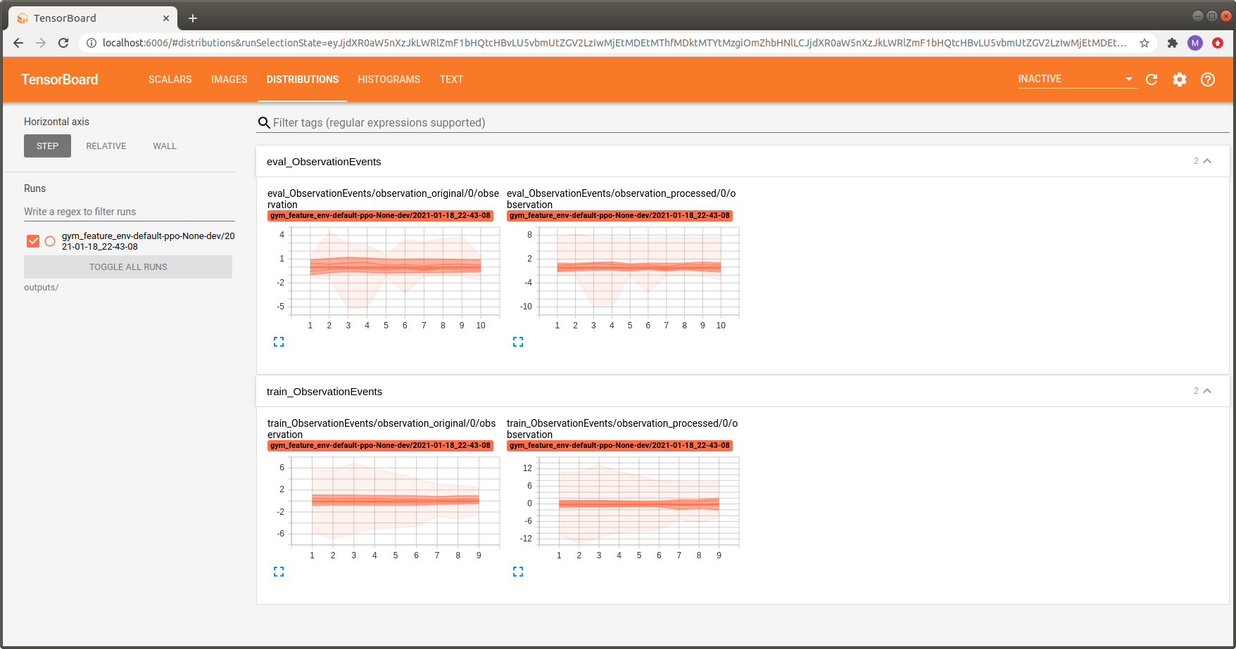
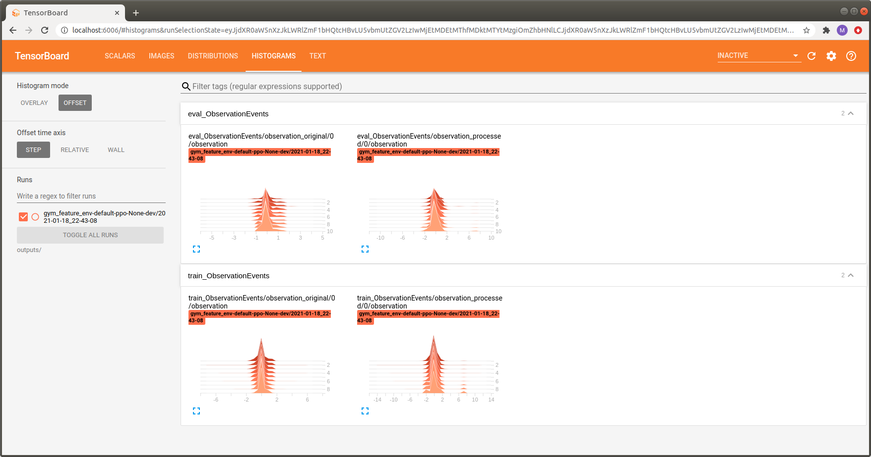
Note that two different versions of the observation distribution are logged:
observation_original: distribution of the original observation returned by the environment.
observation_processed: distribution of the observation after processing (e.g. pre-processing or normalization).
This is useful to verify if the applied observation processing steps yield the expected result.
Observation Visualization
Maze additionally provides the option to directly visualizes observations presented to your policy and value networks as images in Tensorboard.
To activate observation visualization you only have to add the
ObservationVisualizationWrapper
to your environment wrapper stack in your yaml config:
# @package wrappers
maze.core.wrappers.observation_visualization_wrapper.ObservationVisualizationWrapper:
    plot_function: my_project.visualization_functions.plot_1c_image_stack
and provide a reference to a custom plotting function (here, plot_1c_image_stack).
from typing import List, Tuple

import numpy as np
import matplotlib.pyplot as plt


def plot_1c_image_stack(value: List[np.ndarray], groups: Tuple[str, str], **kwargs) -> None:
    """Plots a stack of single channel images with shape [N_STACK x H x W] using imshow.

    :param value: A list of image stacks.
    :param groups: A tuple containing step key and observation name.
    :param kwargs: Additional plotting relevant arguments.
    """

    # extract step key and observation name to enter appropriate plotting branch
    step_key, obs_name = groups

    fig = None
    # check which observation of the dict-space to visualize
    if step_key == 'step_key_0' and obs_name == 'observation-rgb2gray-resize_img':

        # randomly select one observation
        idx = np.random.random_integers(0, len(value), size=1)[0]
        obs = value[idx]
        assert obs.ndim == 3
        n_channels = obs.shape[0]
        min_val, max_val = np.min(obs), np.max(obs)

        # plot the observation
        fig = plt.figure(figsize=(max(5, 5 * n_channels), 5))
        for i, img in enumerate(obs):
            plt.subplot(1, n_channels, i+1)
            plt.imshow(img, interpolation="nearest", vmin=min_val, vmax=max_val, cmap="magma")
            plt.colorbar()

    return fig
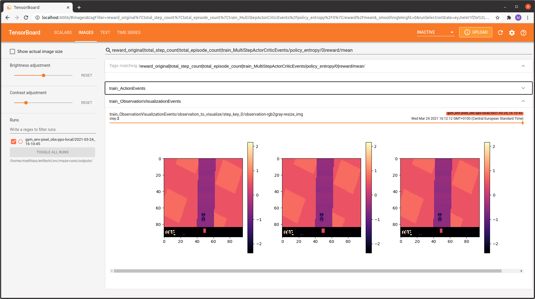
The function above visualizes the observation observation-rgb2gray-resize_img (a single-channel image stack) as a subplot containing three individual images:
Where to Go Next
You might be also interested in logging action distributions.
You can learn more about observation pre-processing and observation normalization.