Action Distribution Visualization
There are situations where it turns out to be extremely useful to watch the evolution of an agent’s sampling behaviour throughout the training process. Looking at the action sampling distribution often provides a first intuition about the agent’s behaviour without the need to look at individual rollouts.
However, most importantly it is a great debugging tool immediately revealing if:
the weights of the policy collapsed during training (e.g., the agent starts sampling always the same actions even though this does not make sense for the environment at hand).
observations are properly normalized and the weights of the policy are initialized accordingly to result in a healthy initial sampling behaviour of the untrained model (e.g., each discrete action is taken a similar number of times when starting training).
biasing the weights of the policy output layer results in the expected sampling behaviour (e.g., initially sampling an action twice as often as the remaining ones).
the agents actually starts learning (i.e., the sampling distributions changes throughout the training epochs).
To activate action logging you only have to add the
MazeEnvMonitoringWrapper
to your environment wrapper stack in your yaml config:
# @package wrappers
maze.core.wrappers.monitoring_wrapper.MazeEnvMonitoringWrapper:
    observation_logging: false
    action_logging: true
    reward_logging: false
Action sampling distributions are then visualized on a per-epoch basis in the IMAGES tab of Tensorboard. By using the slider above the images you can step through the training epochs and see how the sampling distribution evolves over time.
Discrete and Multi Binary Actions
Each action space has a dedicated visualization assigned. Discrete and multi-binary action spaces are visualized via histograms. The example below shows an action sampling distribution for the discrete version of LunarLander-v2. The indices on the x-axis correspond to the available actions:
Action \(a_0\) - do nothing
Action \(a_1\) - fire left orientation engine
Action \(a_2\) - fire main engine
Action \(a_3\) - fire right orientation engine
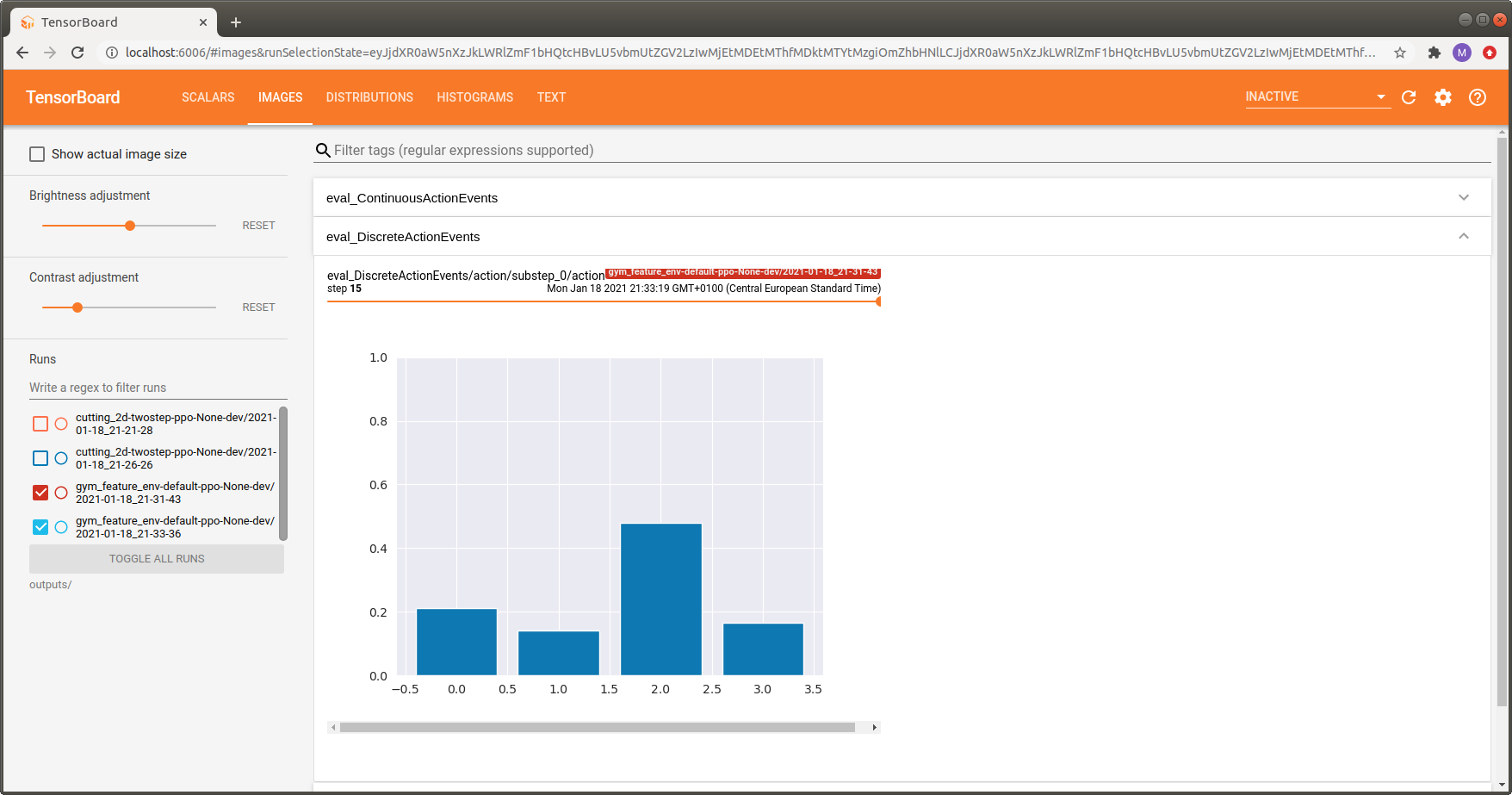
We can see that action \(a_2\) (fire main engine) is taken most often, which is reasonable for this environment.
Continuous Actions
Continuous actions (Box spaces) are visualized via violin plots. The example below shows an action sampling distribution for LunarLanderContinuous-v2. The indices on the x-axis correspond to the available actions:
Action \(a_1\) - controls the main engine:
\(a_1 \in [-1, 0]\): off
\(a_1 \in (0, 1]\) throttle from 50% to 100% power (can’t work with less than 50%).
Action \(a_2\) - controls the orientation engines:
\(a_2 \in [-1.0, -0.5]\): fire left engine
\(a_2 \in [0.5, 1.0]\): fire right engine
\(a_2 \in (-0.5, 0.5)\): off
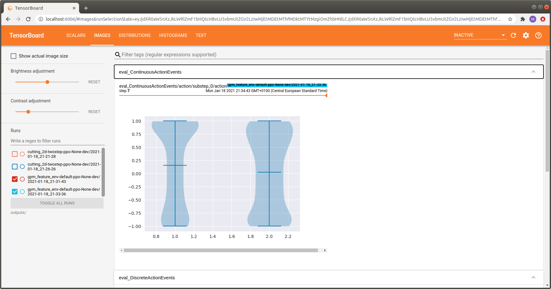
For the first action, corresponding to the main engine, values closer to 1.0 are sampled more often which is similar to the discrete case above.
Where to Go Next
You might be also interested in logging observation distributions.